This text is an offprint of Chapters 22 to 27 of the book concerning the cycle of crises in the United States since 1929[1]. The chapters deal with the cycle of fixed capital and demonstrate mathematically that the reproduction of fixed capital and variations in it lead to a wave that has the same length as the period of the turnover of fixed capital.

This demonstration therefore provides a solid basis for Marx’s preliminary remarks regarding the impact of the variations in fixed capital accumulation on the cycle. These variations are permanent, but the most important ones become apparent when crises break out. The demonstration that the reproduction of fixed capital contains a cyclical element with a length of the cycle corresponding to the turnover period of fixed capital provides us with a basis for Marx’s perspective regarding the relationships between the cycle and the reproduction of fixed capital.

Nevertheless, it would be erroneous[2] to make this reproduction of fixed capital into a preponderant factor in the cycle as it is, as Marx remarked, just a single element, one of the material bases. It could also be thought at the end of this demonstration that it plays an independent role. By affecting the cycle at the end of the turnover period of fixed capital, the previous major variation could contribute to deepening, or accentuating the crisis, if other factors resulting from the cycle of accumulation, the financial cycle etc., are ready to make the crisis break out; or otherwise, if the cycle either lasts beyond, or alternatively, falls short of the period of turnover of fixed capital, the wave produced by the variations in accumulation of fixed capital would play a role in it of the same kind, but with a minor effect.

We know little about the period of turnover in the current period. How long does it last? Does it have a relatively fixed nature? Does it tend to become shorter?

As we explained in Chapter 7 of the book on the cycle of crises in the United States, we were unable to show from the statistics the effects of the cycle of fixed capital[3]. In fact, we had not found a method for establishing from the statistics what the demonstration proposed. Perhaps comrades who are cleverer than us will be able to do so. It is above all for this reason that we are publishing separately this offprint.

2. Theoretical analysis: presentation of the problem

2.1 A difficult question that is easy to set aside

“Scores of authors try to defend this policy [of artificially lowering interest rates by credit expansion] by producing spurious explanations of the trade cycle and by passing over in silence the monetary theory. As they see it, the recurrence of economic crisis is inherent in the very nature of the unhampered market.

The originator of this fallacy was Karl Marx. It is one of the main dogmas of his teachings that the periodical return of commercial crises is an inherent feature of the “anarchy of production” under capitalism. Marx made various lame and contradictory attempts to prove his dogma; even Marxian authors admit that these ventures were utterly futile.” (Ludwig von Mises “Economic Freedom and Interventionism” – Review of Alvin H. Hansen Business Cycles and National Income – in “The Freeman”, September 24, 1951. Available at: https://mises.org/library/economic-freedom-and-interventionism/html/p/136)

This is how one of the strongest defenders of laissez-faire spoke out in 1951. Today, clearly, after so many crises, above all that in 2008-2009, we can only pityingly smile when coming across such imbecilic fanaticism, while Marx’s theory scores a new overwhelming victory.

A theory concerning the origins of the cycle nevertheless does not emerge on its own, and the Italian left could make an ironical statement at the same time that Ludwig von Mises was crapping on with his insults:

“The difficult problems of the framework of the economic cycle which racked the brains of the schoolboys such as the Quesnays, Sismondis and Marxs, become child’s play. The key to them is the customer, the King of wealth, just as the citizen is the King of power. It does not matter a hoot if he is a simple wage labourer, a salaried clerk or a petit bourgeois: as Charles V shouted to the peasants of Alghero “estate todos caballeros!”[4], American high finance shouts to people worldwide “estate todos clientes!”[5], the highest rank of nobility in the mercantile economy” (Il proletariato cliente. Politica economica USA-pacchiana… Battaglia comunista, no. 1, 1952).

This intrinsic difficulty concerning the question of the cycle, also with the incompleteness, as we shall see, of Marx’s reflection on the subject, has led certain Marxists to brusquely set aside any attempt to go into the problem in depth and instead falsify Marx’s own point of view. A typical representative of this way of seeing things is found in Paul Mattick when he states in his book Marx and Keynes:

“The definite crisis-cycle of the last century is, however, an empirical fact not directly related to Marxian theory. It is true that Marx tried to connect the definite periodicity of the crisis with the turn-over of capital. But he did not insist on the validity of this explanation. In any case, his theory does not depend on any particular periodicity of crises. It only maintains that crises are bound to arise as an expression of the temporary overproduction of capital and as the medium for the resumption of the accumulation process.” (Paul Mattick, Marx and Keynes, Merlin, p. 73)

2.2 The cycle of crises lies at the heart of the forecast

Even though it may displease bourgeois thought and revisionism, the analysis of cycles and their periodical nature lies at the heart of the revolutionary perspective of Marxism. Right from the start, right from the embryonic conception, we could say[6], of the materialist conception of history, this study of the crisis has been at the very heart of the forecast regarding both the catastrophic course of the capitalist mode of production and the revolutionary action that could arise from it.

Engels in his 1845 book on the working classes in England already foresaw two new crises, which should have led on to the victory of the proletariat[7]. Only the first forecast was to be crowned with success and the revolutionary movement, peaking in 1848, was defeated. It was the counter-revolution and not the revolution to emerge victorious. The founders of scientific socialism therefore formed an interest in the cycle of crisis from the moment of its gestation.

Such considerations for them had an immediate practical character. The check to the revolutions in 1848 and their defeat in one country after another led Marx to think that the counter-revolution was needed for the proletariat to dispel its last illusions and prepare itself for a new revolutionary wave. This should not have failed to take place about five years after the 1847 crisis on the occasion of a new economic crisis which should have shaken capitalist production.

Marx and Engels thus worked out at the beginning of 1850 a cycle of crises of about five years. This analysis was seemingly not yet based on solid theoretical conceptions, but on the use of empirical evidence that showed that crises had taken place about every five years since 1825. They quickly realized that this perspective was incorrect[8]. The facts disproved Marx and Engels forecast as the crisis were taking place at greater intervals. The cycle Marx witnessed had lasted about ten years by then. This did not lead Marx to abandon the idea that crises were periodic, quite the contrary. He spent all his life searching for the roots of crises and in forecasting their reappearance, using mathematical methods too. Marx and Engels used this episode to form the idea that there were intermediate crises within the cycle of general crises, and these intermediate crises, if they were strong enough, could lead to pre-empting the general crisis[9]. Later on, Engels will consider that these intermediate crises had disappeared[10]. As we have seen, above all with case of cycles in waves[11], while, on one hand, the idea of intermediate crises, when they existed, could pre-empt the general crisis is always valid (the case of the 8^th cycle is particularly significant)[12]. On the other hand, intermediate crises form part of the tendency towards stagnation, which then translates into a lengthening of the cycle. Frequency and intensity have tended to be inversely related[13]. Since the time capital mustered its productive forces; its cycle has shortened and, inversely, the tendencies to stagnate have led to the lengthening of the cycle.

2.3 The search for one of the material bases of the cycle of crises

Marx looked for one of the material bases of the cycle of crises in the turnover time of fixed capital following the long-awaited crisis, which did not break out until 1857[14].

“A propos. Can you tell me how often machinery has to be replaced in, say, your factory? Babbage maintains that in Manchester THE BULK OF MACHINERY IS RENNOVATED ON AVERAGE EVERY 5 YEARS. This seems to be somewhat STARTLING and not QUITE TRUSTWORTHY. The average period for the replacement of machinery Is one important factor in explaining the multi-year cycle which has been a feature of industrial development ever since the consolidation of big industry.” (Marx to Engels, 2/3/1858, in Collected Works, Vol. 40, p. 278)

Engels’ reply seemed to be satisfactory and suggested to Marx to make the following comments:

“The figure of 13 years corresponds closely enough to the theory, since it establishes a unit for ONE EPOCH OF INDUSTRIAL REPRODUCTION which plus ou moins coincides with the period in which major crises recur; needless to say their course is also determined by factors of a quite different kind, depending on their period of reproduction. For me the important thing is to discover, in the immediate material postulates of big industry, one factor that determines cycles.” (Marx to Engels, 5/3/1858, in Collected Works, Vol. 40, p. 282)

These extracts show us, apart from the efficient operation of the postal service at the time, the theoretical orientation Marx adopted and maintained for the rest of his life, despite certain reserves on Engels’ part. Marx, in fact, returned to the subject in August 1862. He was interested in the difference between reproduction in value and reproduction in nature of fixed capital.

“AT ALL EVENTS, in the course of those 12 years does not 1/12 of the machinery have to be replaced in natura each year? Now, what becomes of this fund, which yearly replaces 1/12 of the machinery? Is it not, in fact, an accumulation fund to extend reproduction aside from any CONVERSION OF REVENUE INTO CAPITAL? Does not the existence of this fund partly account for the very different rate at which capital accumulates in nations with advanced capitalist production and hence a great deal of capital fixe, and those where this is not the case?” (Marx to Engels, 20/8/1862, in Collected Works, Vol. 41, pp. 411-412)

Engels, who had just before received the famous letter on production price and absolute rent, dissuaded him from continuing with the line of research.

“Likewise, the question of wear and tear where, however, I rather suspect you have gone off the rails.” (Engels to Marx, 9/9/1862, in Collected Works, Vol. 41, p. 414)

Marx posed the problem to his friend again five years later:

“Many years ago I wrote to you that it seemed to me that in this manner an accumulation fund was being built up, since in the intervening period the capitalist was of course using the returned money, before replacing the capital fixe with it. You disagreed with this SOMEWHAT SUPERFICIALLY in a letter. […] Now, as a manufacturer, you must know what you do with the RETURNS on capital fixe before the time it has to be replaced in natura. And you must answer this point for me (without theorizing, in purely practical terms).” (Marx to Engels, 24/8/1867, in Collected Works, Vol. 42, p. 408)

Now Marx felt sufficiently convinced about the cycle of crises to wrote in the only part of “Capital” (the first volume) published during his life:

“Just as the heavenly bodies always repeat a certain movement, once they have been flung into it, so also does social production, once it has been flung into this movement of alternative expansion and contraction by a mechanical necessity. […] only after all this [the most modern capitalist mode of production – ed.] had happened can one date the repeated self-perpetuating cycles, whose successive phases embrace years, and always culminate in a general crisis, which is the end of one cycle and starting-point of another. Until now the duration of these cycles has been ten or eleven years, but there is no reason to consider this duration as constant. On the contrary, we ought to conclude, on the basis of the laws of capitalist production as we have just expounded them, that the duration is variable, and that the length of the cycles will gradually diminish.” (Marx, Capital Vol. 1, Penguin, p. 786)

Even if only a few explanations are offered by Marx, (he was never to give many others) for the relations between the cycle of crises and the reproduction of fixed capital, he remained convinced right through to his last manuscripts. In Capital Volume 2, the last of the three he wrote, which all the same contains an analysis of simple reproduction of fixed capital, which does not allow for the appearance of any contradiction in the process of reproduction, Marx nevertheless states:

“One may assume that in the essential branches of large-scale industry this life cycle [of fixed capital – ed.] now averages ten years. However, we are not concerned here with the exact figure. This much is evident: the cycle of interconnected turnovers embracing a number of years, in which capital is held fast by its fixed constituent part, furnishes a material basis for the periodic crisis. During this cycle, business undergoes successive periods of depression, medium activity, precipitancy, crisis. True, periods in which capital is invested differ greatly and far from coincide in time. But a crisis always forms the starting-point of large new investments. Therefore, from the point of view of society as a whole, more or less, a new material basis for the next turnover cycle.” (Marx, Capital Vol. 2, Collected Works, Vol. 36, pp. 187-188)

The question asked in this research, which was uninterrupted and never brought to a conclusion, is the following: does the reproduction of fixed capital contain a contradiction that can serve as an element able to explain the cycle of crises?

If such a contradiction had a material basis, it would be necessary to provide it with a mathematical expression. In this way, the fact that the reproduction of fixed capital contains a cyclical element would be proved. Moreover, it would be necessary to show that this cyclical element is related to the period of the turnover of fixed capital in order to corroborate Marx’s perspectives.

Fixed capital also contains another factor in the crisis that we will not try to develop on here. It is linked to the importance of the period of production of fixed capital. The production and accumulation of fixed capital whose period of production is lengthy (major infrastructure, works of art etc.) requires the achievement of a high level of labour productivity. The possibility, as well as the necessity, of finding an outlet able to limit overproduction presupposes, if this type of production is to be executed, the existence of a population that can free itself from immediate production. Furthermore, all things being equal, the longer the period of production, the greater the sum of capital advanced. Time will pass between the moment when fixed capital of this type begins to be installed and the moment when it can be used. Capital has to be advanced throughout this period. It allows for the immobilization of capital in the production of a fixed capital which will only have a future effect on social productivity and, from this point of view, play a role in limiting overproduction. On the other hand, these major payments of advanced capital suppose a relative surplus which can only exist when there is a basis of high labour productivity. This type of production is also a permanent factor in the crisis. These crises are not general crises of overproduction, but disproportions instead. These disproportions between fixed and circulating capital are because the variations created in the production of fixed capital (whose period of reproduction they help to lengthen) play a role in the periodicity of the cycle[15].

3. The divergence between mass and value of fixed capital

3.1 The reproduction of fixed capital

Let us take up the matter where Marx left off. The questions he asked Engels regarded the difference between the renewal of capital in kind and the transfer of the value of fixed capital to the product. The renewal of a fixed capital in kind takes place when it can no longer operate. Physical depreciation is the final limit for its use, its “moral” amortization, its obsolescence, be it planned or not, is more generally the reason for its renewal. Like any other constant capital, fixed capital has the sole function of transferring its value to the product.

3.2 Numerical example

Let us presume that in society there is, at time t₀, a fixed capital of the value C₀, with the value 1,000 representing a mass M₀ of use value of whatever consistency, for example 1,000 units of machines of the same type (we are offering an abstraction of the discrete character of the use value).

Let us suppose that the turnover time of the fixed capital is equal to r, that is, the fixed capital transfers its entire value to the commodities produced in r years. For our example, we pose r = 2 years.

If each year the fixed capital is accumulated at the rate g (10% in our example), this means that, in our particular case, the mass of machines accumulated would be 1,100 in the following year (t₀₊₁)[16].

On the other hand, as we have posed a unit value constant over time for each machine equal to 1, the mass of machines accumulated in t_0-r (r years before t₀) was:

Where M₀ is the mass of fixed capital, the number of machines, at time t₀. In our example, M₀=1,000, while the rate of accumulation of fixed capital is g = 0.1 and the turnover time r is two years (r = 2). With r = 2, this formula says that M₀ (1,000) results from the accumulation of fixed capital throughout the years t_0-2 and t_0-1.

If we insert these data in the equation below, the mass of fixed capital, the number of machines, accumulated in time t_0-2 was:

The value of the fixed capital is transferred by the action of living labour to the value of the commodities. The transfer of this value takes place in each turnover time prorates for the length of the turnover of fixed capital (r being 2 in our example).

In time t_0,when the value of fixed capital is 1,000, the value transferred to the commodity product will therefore be 500 because the turnover time of the fixed capital is two years. In other words, it transfers the full value in two years. The equation is therefore where v is the unit value of the fixed capital (1 in our example).

For the same reason, the value transferred in t_0-1and in t₀by the fixed capital accumulated in t_0-2would be equal to:

In our example, the value of fixed capital transferred to the product in t_0-1and t₀is therefore 476.19/2 = 238.1.

In our example, the actual mass (t₀) of fixed capital is the result of the last two years of accumulation of fixed capital since the turnover period lasts two years. We have calculated the mass of fixed capital accumulated in t_0-2and we could do the same for the capital accumulated in t_0-1. We know that the rate of accumulation of fixed capital is g, so consequently the mass of fixed capital accumulated in t_0-2is equal to:

In our example: 476.19 (1 + 0.1) = 523.8

Seeing that the unit value of this fixed capital is 1, the value of the fixed capital accumulated in t_0-1would therefore be 523.8.

The mass of fixed capital in t₀is the result of two generations of fixed capital: the fixed capital accumulated in t_0-2and the fixed capital accumulated in t_0-1. The mass of fixed capital therefore equals 476.2 + 523.8, being 1,000 units of fixed capital. It is not the same case for the value of the fixed capital. This is equal to 476.2/2 + 523.8 being 761.9 (half of the value of the fixed capital accumulated in t_0-2transferred its value to the product in t_0-1).

What happened with the accumulation of fixed capital in year t₀?

The machines accumulated during the year t_0-2are taken out of production after having transferred the rest of their value to the social product at the same time. Consequently, 476.2 machines are taken out of production while the value transferred to the product rises to 238.1. In order to obtain the whole of the value transferred to the product due to the progressive amortization of fixed capital, we have to add that provided by the machines installed more recently and which still remain in operation, but whose value falls by half, that is 523.8/2 = 261.9. The total value of fixed capital transferred to the social product during year t₀is therefore equal to 238.1 + 261.9 = 500.

If the accumulation of fixed capital at the rate of 10% continues, the mass of new fixed capital accumulated would rise to 523.8 * 1.1 = 576.18. Like the mass fixed capital scrapped, the generation accumulated in t_0-2comes to 476.2, the total mass of fixed capital rising from 1,000 to 1,100 (523.8 + 576.2 – 476.2). On the other hand, the net value of the fixed capital accumulated equals 838.1 (576.2 + 261.9). The net value of the capital accumulated also rises by 10%; the net value of fixed capital has risen by 76.2, that is, 10% of the previous value of the fixed capital (761.9). The unit value of fixed capital being 1, means that an additional value of 76.2 allows for an increase in the mass of machines of only 76.2 units, while the mass required in order to increase by 10% the mass of fixed capital is 10% of 1,000, that is 100. There is a divergence between the increase of the value of the fixed capital and the increase in its mass. The increase in value results exclusively from accumulation, while the increase in the mass is realized not only by the accumulation, but also by the role of simple reproduction of fixed capital.

We have seen that in t₀the value of fixed capital transferred to the product stood at 500. This value, which corresponds to the simple reproduction of fixed capital, allows for the purchase of 500 units of fixed capital, 500 machines, while only 476.2 are now out of service. An increase follows in the mass of fixed capital of 23.8 (500 - 476.2) units for the simple operation of the simple reproduction of fixed capital. If we add on to these 23.8 units, coming from the simple reproduction of fixed capital, to the 76.2 produced by accumulation, the total number of machines rises by 100 (76.2 + 23.8) units. For its part, the value of the fixed capital rises by 10%, or 76.2, but only thanks to the accumulation of surplus value.

3.3 General formula

In our example, therefore almost 24% (23.8/100) of the rise in the mass of fixed capital is due to its simple reproduction. What is the general formula?

Provided the equality of use value and exchange value, supposing that the unitary value of fixed capital is constant, the share due to simple reproduction of fixed capital in the growth of its mass equals:

We can simplify the equation by dividing each term by

This equation defines which share of the accumulation of the mass of fixed capital is due to simple reproduction of it due to the difference existing between the value of fixed capital transferred to the product and the value of the mass of fixed capital definitely destroyed each year.

In our example, g = 0.1 and r = 2, thus

= 23.8%

If the turnover time of fixed capital was 3 for a rate of accumulation of 10%, we would reach this result.

= 31.2%

4. The relationships mass value

4.1 The trend of the share of simple reproduction: numerical example

The preceding example allows us to state that the share devolved to simple reproduction of fixed capital plays a variable role in the mass of fixed capital accumulated.

What is the trend of this share for a given rate of accumulation (g) when the turnover time of fixed capital (r) varies?

Let us take the general formula:

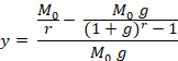
For example, when g = 20% we get the following table:

g	r	y
20%	2	22.7%
20%	3	29.3%
20%	4	31.8%
20%	5	32.8%
20%	6	32.9%
20%	7	32.7%
20%	8	32.2%
20%	9	31.5%
20%	10	30.7%

Using the data calculated, we can draw the following graph:

In this example, where the rate of accumulation of fixed capital is 20%, the curve peaks at a turnover time of fixed capital of about 6 years. At this moment, the share of simple reproduction of fixed capital represents about a third of the accumulation of the mass of fixed capital.

4.2 General equation

We are interested in finding the maximum value of r for a given g in the general formula. To avoid the mathematical complexities involved on the analysis of each curve that allows us to find such values, we informally observe that this family of curves always have a peak within a chosen large range of values of r and g. This being said, the maximum value of r is reached when the derivative of the general formula with respect to r is zero (always assuming g as a constant).

We therefore have to obtain the derivative of the equation, that is to say:

What is this derivative equal to?

The derivative of a difference is equal to the difference of its derivatives.

So the derivative of y, being y’, is equal to the derivative of minus the derivative of

The derivate of with respect to r is equal to (the derivative of a function type is equal to and, as g is a constant, its derivative is zero)

The second term is also of type and so the derivative is equal to

Here

The derivate u’ of u is more complex. It breaks down into two members which form a difference. Being and 1.

1 is a constant and therefore its derivative is zero.

We still have to calculate the derivative of which is an exponential function whose base is .

This type of function has a derivative equal to . Consequently, the derivative u’ is equal to

Thus, the derivative of the second term is therefore:

The derivative of the equation with respect to r is therefore:

When the derivative is zero, assuming our premises, r is at its maximum. Thus r is at its maximum when

The transformation of the previous equation gives:

Then

, or

As we assume g as a constant, this equation can be numerically computed.

4.3 The maximum of the relationship between the rate of accumulation and the turnover time of fixed capital

Since g tends to 0, the maximum share of simple reproduction in the accumulation of the mass of fixed capital is obtained for an ever-increasing value of r.

For example, when g stands at 5%, the derivative is zero when r stands at about 11 years against approximately 6 years when g stands at 20%.

The table below gives the positive values of r for a given value for g computed from the general equation above, and thus allows us to obtain a maximum share for simple reproduction in the accumulation of the mass of fixed capital.

g	r	g	r	g	r
0,50%	34,7	7,50%	9,1	19%	5,9
1%	24,5	8%	8,8	20%	5,8
1,50%	20,1	8,50%	8,6	25%	5,3
2%	17,4	9%	8,4	30%	4,9
2,50%	15,6	9,50%	8,2	40%	4,3
3%	14,3	10%	8	50%	4
3,50%	13,2	11%	7,6
4%	12,4	12%	7,3
4,50%	11,7	13%	7,1
5%	11,1	14%	6,8
5,50%	10,6	15%	6,6
6%	10,2	16%	6,4
6,50%	9,8	17%	6,2
7%	9,4	18%	6,1

We can draw the following graph using these data. It links the maximum for the turnover time to a given rate of accumulation of fixed capital.

4.4 The trend of the maximum of simple reproduction in the rate of accumulation of the mass of fixed capital

We showed in Chapter 4.1 how, with the variation of the turnover time of fixed capital, the share of simple reproduction changes for a rate of accumulation (g) of the given magnitude of fixed capital.

Starting from the results contained in Chapter 4.2, we can determine the maximum share represented by the simple reproduction of fixed capital in the process of reproduction on an extended scale of the mass of fixed capital.

The starting equation was:

How does this equation change for the maximum r for different rates of growth?

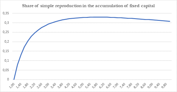
If we replace in the above equation g and r by values obtained from the calculation of the maxima, we obtain the following table and graph:

g	r	Share of simple reproduction	g	r	Share of simple reproduction
0,5%	34,7	47,1%	9%	8,4	38,2%
1%	24,5	45,9%	9,5%	8,2	37,8%
1,5%	20,1	45,0%	10%	8,0	37,6%
2%	17,4	44,3%	11%	7,6	37,0%
2,5%	15,6	43,6%	12%	7,3	36,5%
3%	14,3	43,0%	13%	7,1	36,0%
3,5%	13,2	42,5%	14%	6,8	35,5%
4%	12,4	42,0%	15%	6,6	35,0%
4,5%	11,7	41,5%	16%	6,4	34,6%
5%	11,1	41,0%	17%	6,2	34,2%
5,5%	10,6	40,6%	18%	6,1	33,8%
6%	10,2	40,2%	19%	5,9	33,4%
6,5%	9,8	39,8%	20%	5,8	33,0%
7%	9,4	39,5%	25%	5,3	31,3%
7,5%	9,1	39,1%	30%	4,9	29,8%
8%	8,8	38,8%	40%	4,3	27,4%
8,5%	8,6	38,5%	50%	4,0	25,4%

Consequently, with a maximum ”r” of a given “g”, the share of the accumulation of the mass of fixed capital which results from its simple reproduction continues to fall with the rise in the rate of accumulation. For example, this share falls from over 47% of the increase of the mass of fixed capital at a rate of 0.5% to less than 33% when the rate of accumulation is 20%.

If we limit the definition domain of the curves studies to bounds compatible with the general reality of the economy, it still remains clear that simple reproduction of fixed capital plays a very important role in total accumulation.

The rate of accumulation of fixed capital depends, on the one hand, on the rate of profit, and, on the other hand, on the rate of accumulation of surplus value. The tendency of the rate of profit to fall would lead especially to a fall in the rate of accumulation of fixed capital. However, this tendency is counterbalanced by the fact that fixed capital represents a growing part of the social product. The fall in the rate of profit and the increase in the rate of accumulation of fixed capital are therefore not incompatible, up to a certain point.

When the rate of accumulation of fixed capital (g) falls, the maximum turnover time of fixed capital (r) rises. The development of technical progress and the accompanying devalorization of capital (either due to rise in productivity in reproducing this fixed capital, or due to its obsolescence) means we must expect that the course of capitalist production goes hand in hand with a shortening of the turnover time.

The supposition that a large part of the accumulation of the mass of fixed capital due to simple reproduction is an advantage for capitalist production, notably by ensuring it a greater stability, is only the case if g and r work one against the other to obtain this optimum. Obtaining the optimum for a given rate of growth would thus always become more difficult with the advance of the capitalist mode of production.

At the same time, the variations in the rate of accumulation of fixed capital are of sufficient magnitude for the former never to be, if not by pure chance, in relation to the corresponding optimal turnover time. We infer that the stability of the turnover time of fixed capital is greater than that of the rate of accumulation of fixed capital. Furthermore, even with great differences in the rate, the share of simple reproduction remains high. Lastly, the area of value around the maximum is large enough[17] for us to be able to conclude that the effects of a divergence between the movements, that are judged to be favourable, of g and r, are of minor importance.

5. The cyclical element in simple reproduction

5.1 Numerical example

We stressed in previous chapters a peculiarity of reproduction on an extended scale of fixed capital by showing the importance of simple reproduction in the accumulation of the mass of fixed capital. Can the divergence between the value of fixed capital transferred to the social product and its replacement in kind contain a cyclical element?

In order to obtain some kind of reply to this question, we presume that the accumulation of fixed capital though the accumulation of surplus value halts. In this case, how do the mass and the value of fixed capital evolve?

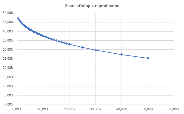
Let us use the following example: the accumulation of fixed capital has risen at a rate of 20% during the turnover time of fixed capital lasting six years, which, as we have seen, is more or less the optimal state of affairs.

Let us assume that there is a mass of fixed capital of 1,000 units with a total value of 1,000. This mass can be broken down in line with date at which the capital was accumulated, into 100.7 units accumulated in t_0-6, 120.85 in t_0-5, 145.01 in t_0-4, 174.02 in t_0-3, 208.82 in t_0-2and 250.59 in t_0-1. Henceforth, as there is no longer surplus value accumulation, there is only the simple reproduction of fixed capital.

At the time of t₀, 100.7 units of fixed capital were used up, such that the replacement of fixed capital allows for an increase in the mass of fixed capital amounting to 166.7 (1,000/6) since the value transferred to the product is 1,000/6. Thus, seeing that the value of fixed capital remains at 670.2, the mass of fixed capital rises to 1,066 in t₀₊₁. The same process continues in t₀₊₂ and reaches a maximum in t₀₊₄, as can be seen in the table and the graph below:

t_0-6	t_0-5	t_0-4	t_0-3	t_0-2	t_0-1	Total	Year
100,71	120,85	145,01	174,02	208,82	250,59	1000	0
120,85	145,01	174,02	208,82	250,59	166,70	1066	1
145,02	174,02	208,82	250,59	166,70	177,70	1123	2
174,02	208,82	250,59	166,70	177,70	187,14	1165	3
208,82	250,59	166,70	177,70	187,14	194,16	1185	4
250,59	166,70	177,70	187,14	194,16	197,52	1174	5
166,67	177,70	187,14	194,16	197,52	195,63	1119	6
177,70	187,14	194,16	197,52	195,63	186,87	1139	7
187,74	194,16	197,52	195,63	186,87	189,77	1152	8
194,16	197,52	195,63	186,87	189,77	191,78	1156	9
197,52	195,63	186,87	189,77	191,78	192,55	1154	10
195,63	186,87	189,77	191,78	192,55	192,28	1149	11
186,87	189,77	191,78	192,55	192,28	191,41	1145	12
189,77	191,78	192,55	192,28	191,41	190,71	1149	13

The mass of fixed capital falls from a maximum of 1,185 to reach a minimum of 1,119 in t₆, always remaining above 1,000. This minimum has a date corresponding to the length of the turnover time of fixed capital, being 6 years. Then a new cycle starts, but its dimension is smaller because the maximum reached in the previous cycle is higher than the maximum in the following one (1,185 against 1,155), while the minimum is lower (1,119 against 1,145). The peak and trough are closer and so the variations diminish, but the period remains the same and equal to the turnover time of fixed capital. The always lesser oscillations means that the mass of fixed capital tends to reach a limit at around 1,150 units. The mass of fixed capital has therefore risen by about 15%, while its value remains constant at 670.2. It is clear that such an accumulation in the mass of fixed capital would require, everything else being unchanged, an accumulation of constant circulating capital and variable capital employed in setting to work this supplementary fixed capital.

Nevertheless, the most notable result is the indication that the difference between the reproduction in value and in kind of the fixed capital contains a cyclical element, which corresponds to the length of the turnover time of fixed capital.

5.2 General equation

The equation for the graph given above is a recurrent series where:

For 1 < t <= r

For t > r

With:

= the mass of fixed capital at time t

= Mass of fixed capital at time t₀ when accumulation stops

r = length of the turnover time of fixed capital

g = the rate of accumulation of fixed capital

Albeit complex, the resolution of these equations is quite possible. We can however save the reader from this operation by following Marx’s theoretical course regarding differential calculus, that is, by standing directly at the limit. The main tendency in differential calculus rejects such a jump, which supposes the passage from a quantitative infinite to a qualitative one. However, what mathematicians devoted to “rigour” would reject with horror can perfectly well be accepted by arithmeticians.

So let us make a jump to the limit, a leap into uncertainty, one of the high points in dialectical transitions in the world of mathematics.

We know the limit situation: it is the simple reproduction of fixed capital. In this moment, the stability of reproduction is achieved.

The gross value of fixed capital where we stopped accumulation is 1,000. The distribution of this value, taking into account the period of turnover (r = 6 years in our example) and the rate of accumulation of fixed capital (g = 20% in our example) following the generations of accumulated fixed capital, is given in detail in the second column of the table. This value remains constant and is broken down in the same proportion year by year (cf. the third and fourth columns).

Year	Gross value of fixed capital accumulated	Residual % accumulated value	Part of the generation of fixed capital in the total value	Present net value
t_-0-6	100,70	1/6	1/21	16,78
t_0-5	120,85	2/6	2/21	40,28
t_0-4	145,02	3/6	3/21	72,51
t_0-3	174,02	4/6	4/21	116,01
t_0-2	208,82	5/6	5/21	174,02
t_0-1	250,59	6/6	6/21	250,59
Total	1000	21/6	21/21	670,19

At the limit, simple reproduction is realized, the transition between a situation of reproduction on an expanded scale of the accumulation of surplus value in the form of fixed capital and a situation of simple reproduction, where the whole of the accumulation of surplus value has stopped, is made.

Consequently, when this simple reproduction is achieved, the value remaining in t_0-6 is 670.19/21 = 31.9. This residual value of the mass of fixed capital assumes that the value of this fixed capital at the time of its accumulation was 191.48 (31.9 * 6). This value also corresponds to the mass of fixed capital accumulated, since we have assumed that a unit of fixed capital had the value of 1.

Consequently, as in every year – the case of simple reproduction – the same mass of fixed capital is accumulated, the total mass of accumulated fixed capital is 191.48 x 6 = 1,148.90 that is the limit of the equations of the text. This method makes it easy to work out the complex equation to calculate the limit of the curve.

To obtain this, all that is required is to take the net total value of fixed capital (the value of the remaining fixed capital) at the time when the accumulation of surplus value stops (for example 670.19), multiply it by the period of turnover (in our example 6) and divide it by the expected value for turnover time (in our example 21/6). This formula is simplified to end up by multiplying the remaining value of fixed capital by two times the turnover time of fixed capital divided by the period of turnover of fixed capital + 1.

We thus obtain the gross value limit of fixed capital. All that is required is the division of this gross value limit by the unit value to obtain the mass of fixed capital limit (here the unit value is 1). Consequently, in our example, the mass and the gross value of fixed capital are the same (1,148.9).

Gross value limit = (The value of fixed capital at the moment when the accumulation of surplus value stops) *

The series is equal to .

Consequently, the gross value limit is equal to: Gross value limit = Net value of fixed capital when the accumulation of surplus value stops *

Mass limit = Gross value limit/unit value

The coefficient of the tendency of the mass of fixed capital is therefore in relation to twice the turnover period divided by the sum 1+r.

Consequently, the limit rises with an increase in the turnover time of fixed capital.

What value does this relation tend to reach? We have to calculate the ratio between when r tends to infinity. In this case, the ratio tends to 2.

If the tendency of capital is to shorten the turnover period, in this case this ratio would tend to fall.

We have therefore shown mathematically that the difference between the reproduction in kind and in value of fixed capital contains a cyclical element and that the length of this cycle is equal to the turnover time of fixed capital. This places Marx’s hypotheses on the firmest theoretical foundations.

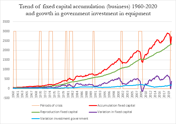
6. The trend of the accumulation of fixed capital

The data available in table 1.15 of the Bureau of Economic Analysis (BEA) show that the accumulation of fixed capital follows the general movement of other forms of capital. In periods called periods of accumulation, the accumulation of capital advances, while in periods of crisis it retreats; fixed capital remains party unused and devalorizes, in various ways, more than in other periods.

We can find data regarding “Saving and Investment” in table 5.1 of the BEA. The data dealing with “domestic business” have been published since 1960; the graphs underline a tendency for crises to worsen. They also refute the idea that “investment”, that is the accumulation of fixed capital, ceased to grow after the 2008-2009 crisis.

The graph below shows the trends of fixed capital. We can see:

- The total amount (in billions of dollars) of accumulated fixed capital. (In red)

- The total derived from the reproduction of this fixed capital (value of fixed capital consumed, in billions of dollars) (In green)

- The difference between the two, which we call variation in fixed capital (in general there is growth). (In violet)

- The difference between government investment in equipment and the part used to renew it. We call this result the variation in government investment (in blue)

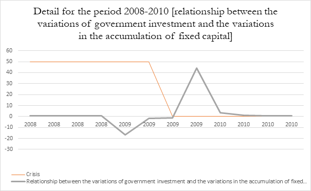
This first graph is followed by a second one, which concentrates on the trend of the relationship between the growth in investment in equipment made by the government (it is not advanced capital, but an outlay of revenue in the form of plant etc.) and the variation in the accumulation of fixed capital by business (as shown in the last two curves of the previous graph). It shows the effects of a so-called “Keynesian” policy[18].

Reasons of space forced us to remove the data for 2009 [and a quarter 2020] from the graphs and provide the details for those years [crisis 2008-2009] separately in the following one.

The variation in the fixed capital of business in 2009 (and the first quarter of 2020) shows disaccumulation, one of the forms of devalorization of capital. The variation is negative and the relationship become negative. This only goes to stress the importance of government action. All the same, even if the graph casts light on the fact that state intervention during the last crisis was the greatest of any cycle, the omission of the data for 2009-2010 greatly weakens the effective representation of this intervention. This has been both relatively[19] and absolutely the greatest since World War Two. Nevertheless, the changes in the relationship are much more secondary than the variations in the accumulation of fixed capital by business than the counter-investment by the state whose amount also appears limited. Furthermore, this graph makes us think that there is a tendency to extend even more greatly state action after the crisis. All the same, that lowest relationship is reached in the present crisis, further proof that capital did not survive the 2008-2009 crisis only because the state held it by the hand.

The cycle that emerges does not offer a forecast[20], but it does corroborate a number of conclusions drawn by the analysis, such as how state intervention during the 1987 financial crisis succeeded in halting the crisis of overproduction; the character of the sixth cycle; the complexity of the fifth cycle etc.

7. Trend of the estimate of the organic composition of capital

We can provide an estimate of the organic composition of capital and follow its trend on the basis of the data available.

It is an estimate as all constant capital has not been taken into account (constant circulating capital is omitted and only the part of fixed capital consumed is given); in wage costs we do not know what part belongs to the production of surplus value.

In theory, the share of fixed capital in constant capital should increase and, if the turnover time of fixed capital diminishes, this could only increase the relative share of fixed capital. Besides, the share of wage earners who do no produce surplus value would tend to rise. Therefore, an increase in the estimate of the organic composition certainly makes us think that the organic composition of capital increases.

The data in table 1.15 of the BEA allows us to produce the following graph[21]:

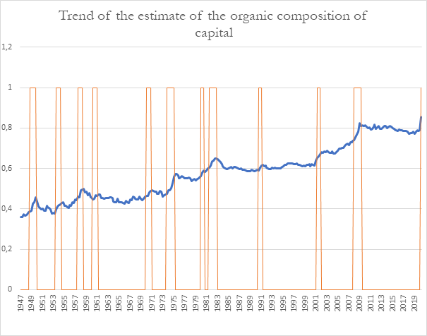
There is a clear tendency to rise. This marks a new theoretical victory for Marxism. This curve also tends to present a cycle, but this is more complex due to the existence of contradictory tendencies. In most cases, the maximum organic composition is reached at the time of the crisis. Nevertheless, this is not always the case and sometimes there is a short slippage (in this case usually a quarter) in relation to the end of the crisis of overproduction. The minimum, and research here is interesting too, is more erratic. Contradictory factors come into play. On the one hand, the recovery of accumulation leads to a better use of fixed capital, and so to a fall in unit prices, on the other hand the accumulation of fixed capital and the rise of the organic composition it entails work in the opposite way. Lastly, wage costs, which are pushed down during the period of crisis, tend to bounce back in the period of accumulation.

[1] Robin Goodfellow, Le Cycle des Crises aux États-Unis depuis 1929 : Essai de systématisation de la conjoncture, L’Harmattan, 2016

[2] See our critique of Marcel Roelandts (cf. the chapter on fixed capital and the crisis) in the book Towards the foundations of the crises – Academic Marxism and Crises.

[3] “Since periods of crisis are also periods of major variations in the accumulation of fixed capital, this leads us to think that they have a special importance in the creation of a periodical wave. However, at the present stage of our research, we have not yet found a method to demonstrate from the statistics the effects of this cycle of fixed capital. If these effects do exist, it would be vital to demonstrate that the variations in the accumulation of fixed capital play a special role at the moment of crises. The accumulation of fixed capital, just as any other capital, falls during the crisis. The challenge is to demonstrate that variations in the accumulation of fixed capital (and the accumulation of capital more generally speaking) depend (and especially at the moment of crises) in part (small, but real) on past variations of the same accumulation of fixed capital.”

[6] “Modern international Socialism, since fully developed as a science, chiefly and almost exclusively through the efforts of Marx, did not as yet exist in 1844. My book represents one of the phases of its embryonic development; and as the human embryo, in its early stages, still reproduces the gill-arches of our fish-ancestors, so this book exhibits everywhere the traces of the descent of Modern Socialism from one of its ancestors, German philosophy.” (Engels, Preface to The Condition of the Working-Class in England (1892) in Collected Works Vol. 27 p. 261.

[7] “The commercial crises, the mightiest levers for all independent development of the proletariat, will probably shorten the process [concentration and centralization of capital, creation of large majority of the proletariat in society – ed.] acting in concert with foreign competition and the deepening ruin of the middle-class. I think the people will not endure more than one more crisis. The next one in 1846 or 1847, will probably bring with it the repeal of the Corn Laws and the enactment of the Charter. What revolutionary movements the Charter may give rise to remains to be seen. But, by the time of the next following crisis, which, according to the analogy of its predecessors, must break out in 1852 or 1853, unless delayed perhaps by the repeal of the Corn Laws or hastened by other influences, such as foreign competition — by the time this crisis arrives, the English people will have had enough of being plundered by the capitalists and left to starve when the capitalists no longer require their services. If, up to that time, the English bourgeoisie does not pause to reflect—and to all appearance it certainly will not do so — a revolution will follow with which none hitherto known can be compared. The proletarians, driven to despair, will seize the torch which Stephens has preached to them; the vengeance of the people will come down with a wrath of which the rage of 1793 gives no true idea. The war of the poor against the rich will be the bloodiest ever waged.” (Engels, The Condition of the Working-Class in England, in Collected Works Vol. 4, pp. 580-581)

[8] “But what purpose this organisation should serve depended very substantially on whether the prospects of a renewed upsurge of the revolution materialised. And in the course of the year 1850 this became more and more improbable, indeed impossible. The industrial crisis of 1847, which had paved the way for the Revolution of 1848, had been overcome; a new, unprecedented period of industrial prosperity had set in; whoever had eyes to see and used them must have clearly perceived that the revolutionary storm of 1848 was gradually declining.

"With this general prosperity, in which the productive forces of bourgeois society develop as luxuriantly as is at all possible within bourgeois relationships, there can be no talk of a real revolution. Such a revolution is only possible in the periods when both these factors, the modern productive forces and the bourgeois forms of production, come in collision with each other. The various quarrels in which the representatives of the individual factions of the Continental Party of Order now indulge and mutually compromise themselves, far from providing the occasion for new revolutions, are, on the contrary, possible only because the basis of the relationships is momentarily so secure and, what the reaction does not know, so bourgeois. All reactionary attempts to hold up bourgeois development will rebound off it just as certainly as all moral indignation and all enthusiastic proclamations of the democrats." Thus Marx and I wrote in the "Review. May to October 1850" in the Neue Rheinische Zeitung. Politisch-ökonomische Revue, No. V-VI, Hamburg, 1850, p. 153” (Engels, On the History of the Communist League, in Collected Works Vol. 26, p. 327-328)

[9] The more the intermediary crises are smoothed out, the deeper the general crisis will be. “I hope that the American PANIC does not get too much out of hand and so have too great a repercussion on England and hence on Europe. General periodic crises are always preceded by such partial ones. If they are too violent they only pre-empt the general crisis and take the sting out of it.” (Marx to Sorge, 25/11/1873, in Collected Works Vol. 44, p. 536)

[10] “The recurring period of the great industrial crisis is stated in the text as five years. This was the period apparently indicated by the course of events from 1825 to 1842. But the industrial history from 1842 to 1868 has shown that the real period is one of ten years; that the intermediate revulsions were secondary and tended more and more to disappear.” (Engels, Preface to The Condition of the Working –Class in England in Collected Works Vol. 27, p. 263)

[11] Cf. Robin Goodfellow, Le Cycle des Crises aux États-Unis depuis 1929 : Essai de systématisation de la conjoncture, L’Harmattan, 2016, 367 pp.

[12] In the above mentioned text, where we analyse the cycles of crises in the US since 1929, we proposed a concept to improve the prediction of crises: the wave of acceleration. Once defined what we call the cycle of rates and ratios (rate of profit, rate of surplus-value, ratio interest over profit…), that is offset from the cycle of crises and allows to refine the prediction of crises, a wave of acceleration is a particular phase of the cycle of the capitalist production which is characterized by the accentuation of the slope of the curve of rates and ratios. The 8^th cycle experienced two waves of acceleration (4^th quarter of 1984-4^th quarter of 1986; 4^th quarter of 1986-3^rd quarter of 1987) before the crisis of overproduction.

[13] A letter from Engels, who was disappointed by the weakness of the current crisis and its slackening, drew Marx’s response “Crisis. By no means burnt out on the Continent (esp. France). Incidentally, what the crises have lost in intensity, they have now gained in frequency.” (Marx to Engels, 4/11/1864 in Collected Works Vol. 42, p. 19)

Marx developed the same idea of crises becoming more frequent in a letter to Lavrov dated 18 June, 1875. “One truly remarkable phenomenon is the decrease in the number of years between general crises. I have always regarded that number not as a constant, but as a decreasing magnitude; what is pleasing, however, is that the signs of its decrease are so palpable as to augur ill for the survival of the bourgeois world.” (Collected Works Vol. 45, p. 78)

[14] In the same period, he wrote in the 1857-1858 Manuscripts (Grundrisse): “There can be no doubt at all that the cycle through which industry has been passing in plus ou moins ten-year periods since the large-scale development of fixed capital, is linked with the total reproduction phase of capital determined in this way. We shall find other determining factors too, but this is one of them. […] But the several-year-long industrial cycle divided up into characteristic periods, epochs, is unique to large-scale industry.” (Marx, 1857-1858 Manuscripts, Grundrisse in Collected Works Vol. 29, p. 105)

[15] Cf. Marx; 1857-1858 Manuscripts, Grundrisse, in Collected Works, Vol. 29, p. 93.

[16] Here, we are interested in a mathematical formulation of the accumulation of fixed capital. For this we will adopt some conventions. To begin with, let us say that t₀ denotes the very starting moment of time of an arbitrary reference year, for example, the first moment of time of January 1, 2021. By the same token, t_0-1 denotes the first moment of January 1, 2020. The same reasoning applies to t_0-2, etc., or t₀₊₁ for the succeeding year (e.g. 2022), and so on. People may generically refer to t₀, t_0-1, t₀₊₁, etc. by their years (e.g. 2021, 2020, 2022), abstracting away their specific moments of time (month, day, hour of a day…). As we are dealing with the turnover time of fixed capital, whose measure is a period of time (one year), and where for a mass of fixed capital functioning in the year t_0-r a part of its value is transferred to the product throughout t_0-r, for the sake of simplicity we say that t_0-r refers to the year corresponding to r years before a reference year t₀. In extenso, this convention means: t_0-r is the year corresponding to r years before a reference year t₀, where one cycle of the turnover time of fixed capital begins at the very first moment of the 1^st January in t_0-r and finishes at the very last moment of the 31^st December in the same year.

[17] For example, in the graph using the example of g = 20%, the share of simple reproduction is above or equal to 30%, with a maximum of 33%, when turnover time lies between 3.2 and 10.9 years.

[18] Even though governments used it even before the birth of Keynes or without taking his advice into account from the time he gave it.

[19] The figures missing are 2009; 1: -16,9; 2009; 2: -1.7; 2009; 3: -1.4; 2009; 4: +44 , 2020 ; 2 . -13.5

[20] It could have been different for the following analysis taken from the article by Auerbach and Gorodnichenko concerning measuring the effects of fiscal policy “Measuring the outpost responses to fiscal policy”: http://www.nber.org/papers/w16311)

[21] All data have been multiplied by 3 to fit onto the page.